Treatment of an Employee’s Gender

When the student researches the gender of employees, a table like the following one will be compiled:

In the table, gender is the research variable. Why variable? Because gender is a characteristic that is not constant for all of the employees. The gender variable for employees can be assigned either of two values: “male” or “female”. The frequency of each value appears in the second column. The number of males in the office appears opposite the value “male”, and the number of females in the office appears opposite the value “female”.

The relative frequency of each value expressed in percentages appears in the third column: The percentage of male employees appears in the row for males and the percentage of female employees appears in the row for females. According to this table, there are 8 male workers in the office constituting 27% of all employees, and 22 female workers in the office constituting 73% of all employees. It is necessary to add another row at the bottom of the frequency table, in which the sums of the columns appear.

We note that in the case of gender, the order of listing in the table is of no significance. The student could have written the females in the first row and the males in the second row. The frequency table can be displayed visually by using a pie chart.

The diagram is called a pie chart because of its round shape. Each value (female and male) receives an area in the pie corresponding to its relative frequency. In our case, the males occupy 27% of the area and the females comprise the remaining 73%. The diagram and the tables answer the question of what the distribution of gender among employees in the office is. The distribution reflects the ratio of males to females among the office employees.

Treatment of Employees’ Marital Status

The same process of statistical treatment of data can also be performed for the marital status section. Marital status is also a variable in which order is of no significance. The marital status variable can be assigned the values “divorced”, “married”, “single”, and “widow/er”. The order among them is unimportant.

We will therefore construct a frequency table in the following manner.

1. We will write these values (divorced, married, single, widow/er) in the first column in any order we please. This is the value column.
2. We will write the frequency of each value (the number of employees) in the second column. This is the frequency column.
3. For each value, we will calculate the proportion that it constitutes of the total quantity of data.
4. We will write the results of the calculation in the third column. This is the relative frequency column.
5. The first two columns:

We calculate the relative frequencies (mouseover the following categories to highlight elements on the chart):

For single: 6/30 = 20%

For widow/er: 1/30 = 3.33%

For divorced: 4/30 = 13.33%

For married: 19/30 = 63.33%

Frequency can also be calculated for the last group (married) by obtaining the sum of 100%. The sum of the percentages of all the first groups is 20% + 3.33% + 13.33% = 36.66%.

In order to total 100%, the percentage of the last group must therefore be 100% – 36.66% = 63.34%

Due to problems in rounding off fractions, there is a slight difference between the two calculations: We obtained 63.33% in the first calculation, and 63.34% in the second. We prefer the second method since all of the relative frequencies will add up to 100% exactly.

We now add the calculations as a third column in the table, and obtain the following frequency table:

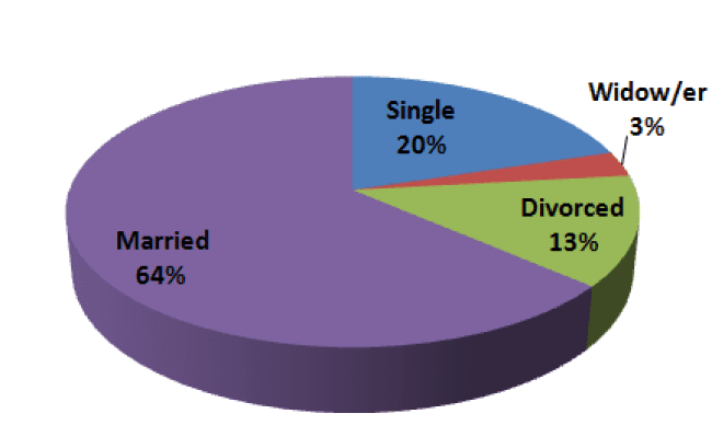
After we have organized the statistical treatment of data in a table, we can present the distribution of marital status by using a pie chart.

This time, the pie will have four “slices”.