Discrete and Continuous Variables

One of the most fundamental properties of variables is their domain. While there is an infinite number of possible domains, they can be divided into two basic classes:

Discrete and Continuous.

Discrete variables describe a finite set of conditions and their values comprise a finite, and usually small, set of values.

Continuous variables can assume an infinite number of values.

While the distinction between discrete and continuous variables is well-defined, the distinction between discrete and continuous quantities is rather vague.

Many quantities can be represented in terms of both discrete and continuous variables.

Discrete variables are usually convenient approximations of real world quantities, which are sufficient for the purpose of projecting the results onto a larger sample.

Treatment of Employees’ Age

The values that are assigned to the age variables are also numerical values. Nevertheless, there is a significant difference between the “Number of children” variable and the “Age” variable.

With the number of children variable, only certain values between the lowest value, 0, and the highest value, 4, can be assigned.

In this case, there are whole numbers only: i.e., 1, 2, or 3, because a situation with 2.78 children, for example, would be impossible. With the age variable, however, between the lowest value, 20, and the highest value, 70, all the values can be assigned. It is possible to be 33.25 years old, or 45.5, or even 27.357. The age variable is therefore called a continuous variable. The “Number of children” variable is called a discrete variable.

Because the number of possible values for a continuous variable is infinite, we will not be able to create a frequency table that will include all of them. We will therefore group the values into divisions: All the employees in their 20s will be placed in the 20 to 30 group, while all those in their 30s will be included in the 30 to 40 group, and so on and so forth. In this case, the divisions actually represent the age groups.

The division appears in the first column of the frequency table, while the frequency, i.e. the number of employees in each age division, appears in the second column.

The relative frequency will appear in the third column.

The following frequency table represents the distribution of the age variable.

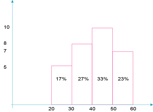
For the visual representation of the distribution of a continuous variable, we will use a histogram

What is a Histogram?

A histogram is a graph comprising adjacent columns. Each division has its own column. There is a column for the 20 to 30 age group, as well as a separate column for the 30 to 40 age group, and so on and so forth. Every column has a specific height and width.

The width of the column is the width of the division, i.e., the range of the division. In our case, the width of each division is 10 because the range of each division is 10 years. There are 10 years between 20 to 30, as well as 30 to 40, and so forth.

How is the height of the column determined? Here we will have to do a short calculation. Since the column has both width and height, it also has an area, i.e., the product of the height multiplied by the width. Statisticians decided that the area of the column would reflect the relative frequency of the age group that it represents. For example, the column width for the 20 to 30 age group will be 10, and the area will be 17. We can therefore calculate the height of the column: 17/10 = 1.7.

The height of the column is called the density.

Before drawing the histogram, we will add two columns to the table: The width of the division (the width of the column) and the density (the height of the column).

The histogram presents the table from the previous page.