We will provide an example to accompany the explanation. This example relates to the height of ten year-old children:

1. A continuous variable – the normal probability distribution reflects the distribution of a continuous variable, which can receive any numerical value, i.e., whole., numbers (for example, 101 centimeters), numbers with fractions (for instance, 101.25 centimeters), positive numbers and negative numbers although there are no negative numbers in our example.
2. The height reflects a probability – the height of the previous curve and every number reflects the chances of that number occurring as compared to the other numbers. The further away we get from the center (either to the left or the right), then the smaller is the chance of the occurrence.
3. The center is the expectation – the center result reflects the average, and the chance of getting it is higher than any other number. The reason why the center result is the average is that the curve is symmetric around the center. This means that for every result to the right of the center that contributes to increasing the average, there is also a result that is at the same distance to the left that has an equal chance of occurring, which contributes an equivalent degree toward decreasing the average.
4. Symmetry – the normal probability distribution is symmetric relative to the average. This means that the chances of obtaining a result exceeding the average by 10 is equal to the chance of receiving a result that is smaller than the average by 10.
5. The probabilities are known in advance.

The probabilities, which are equivalent to the areas under the curve on both sides of the average are distributed as follows:

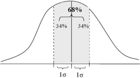
1. Each of the areas above the segment (over the X axis) with a length of one standard deviation (1?) from the average (i.e., one to the right and one to the left) totaling 34% of the area within the normal curve. The area above a segment with a length of 2 standard deviations on both sides of the average (i.e., from 1 standard deviation to the left of the average to 1 standard deviation to the right of it) therefore totals 68% of the area within the normal curve.
   

   Diagram A

   
   
   

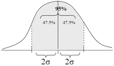
2. Each of the areas above the segment with a length of 2 standard deviations (2?) from the average (i.e., one to the right and one to the left) totals 47.5% of the total area within the normal curve. The area above a segment with a length of 4 standard deviations on both sides of the average (i.e., from 2 standard deviations to the left of the average to 2 standard deviations to the right of it) therefore totals 95% of the total area within the normal curve.
   

   Diagram B

   
   
   

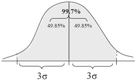
3. Each of the areas above the segment with a length of 3 standard deviations (3?) from the average (i.e., from one to the right to one to the left) totals 49.85% of the total area within the normal curve. The area above a segment with a length of 6 standard deviations on both sides of the average (i.e., from 3 standard deviations to the left of the average to 3 standard deviations to the right of it) therefore totals about 99.7% of the total area within the normal curve.
   

   Diagram C

   

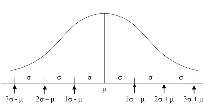
Marking intervals on the X axis

The average is denoted by the Greek letter μ (mu).

The standard deviation is denoted by the Greek letter σ (sigma).

A point 1 standard deviation to the right of the average is denoted by μ + 1σ.

A point 1 standard deviation to the left of the average is denoted by μ1- σ.

The distance between these two points is denoted by μ +/- σ.

In general:

A point X standard deviation to the right of the average is denoted by μ + Xσ.

A point X standard deviation to the left of the average is denoted by μ – Xσ.

The distance between these two points is denoted by μ +/- Xσ.

to the right and one to the left) totals 47.5% of the total area within the normal curve.

The area above a segment with a length of 4 standard deviations on both sides of the average (i.e., from 2 standard deviations to the left of the average to 2 standard deviations to the right of it) therefore totals 95% of the total area within the normal curve.

3. Each of the areas above the segment with a length of 3 standard deviations (3?) from the average (i.e., from one to the right to one to the left) totals 49.85% of the total area within the normal curve.

The area above a segment with a length of 6 standard deviations on both sides of the average (i.e., from 3 standard deviations to the left of the average to 3 standard deviations to the right of it) therefore totals about 99.7% of the total area within the normal curve.

The average is denoted by the Greek letter ? (mu).

The standard deviation is denoted by the Greek letter ? (sigma).

A point 1 standard deviation to the right of the average is denoted by ? + 1?.

A point 1 standard deviation to the left of the average is denoted by ? – 1?.

The distance between these two points is denoted by ? +/- ?.

The Significance of Areas Within the Curve

As noted previously, the areas within the curve represent probabilities. In our example, the probability of finding a child whose height is in the segment between μ – σ and μ + σ is 68%.

In other words:

Of every 1,000 children that we meet in the street, the height of 680 of them (68%) will be within the segment between μ – δ and μ + δ.

Furthermore:

Of every 1,000 children we meet in the street, the height of 950 of them (95%) will be in the segment between μ – 2σ and μ + 2σ, and the height of 997 of them (99.7%) will be in the segment between μ – 3σ and μ + 3σ.

Only 3 of every 1,000 children will be outside the segment between μ – 3σ and μ + 3σ.